Output Data

The main inference results are kept in the composite type DiscreteTreeModel in the subtype DiscreteInference with fields:

fromFactor,
toVariable
messageFactorVariable,
fromVariable
toFactor
messageVariableFactor,
marginal.

The values of messages from factor nodes to variable nodes can be accessed using messageFactorVariable field, while values of messages from variable nodes to factor nodes are stored in messageVariableFactor field. These values correspond to edges defined by factor and variable nodes, with indexes preserved in fromFactor - toVariable and fromVariable - toFactor fields.

Fields marginal holds state variable normalized marginal distributions.

The DiscreteInference field contains the BP algorithm results. To describe the outputs, we will use the example with four random variables, where random variables $\{x_1, x_2, x_3, x_4 \}$ have possible states $\{ 4, 3, 1, 2\}$.

using FactorGraph

probability1 = [1]
table1 = [0.2; 0.3; 0.4; 0.1]

probability2 = [1; 2; 3]
table2 = zeros(4, 3, 1)
table2[1, 1, 1] = 0.2; table2[2, 1, 1] = 0.5; table2[3, 1, 1] = 0.3; table2[4, 1, 1] = 0.0
table2[1, 2, 1] = 0.1; table2[2, 2, 1] = 0.1; table2[3, 2, 1] = 0.7; table2[4, 2, 1] = 0.1
table2[1, 3, 1] = 0.5; table2[2, 3, 1] = 0.2; table2[3, 3, 1] = 0.1; table2[4, 3, 1] = 0.1

probability3 = [4; 2]
table3 = zeros(2, 3)
table3[1, 1] = 0.2; table3[2, 1] = 0.8
table3[1, 2] = 0.5; table3[2, 2] = 0.5
table3[1, 3] = 0.5; table3[2, 3] = 0.5

probability4 = [4]
table4 = [0.4; 0.6]

The factor graph construction and message initialization is accomplished using discreteTreeModel() function.

probability = [probability1, probability2, probability3, probability4]
table = [table1, table2, table3, table4]

bp = discreteTreeModel(probability, table)

Factor graph and root variable node

The first step in solving/analysing the above system/system of equations is forming a factor graph, where set of variable nodes $\mathcal{X} = \{x_1, x_2, x_3, x_4 \}$ is defined by discrete random variables. The set of conditional probability tables denotes the set of factor nodes $\mathcal{F} = \{f_1, f_2, f_3, f_4\}$. Here, we leave the default setting for the root factor, or the function discreteTreeModel() sets the first variable node $x_1$ as the root node.

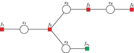
Figure 1: The tree factor graph with three variable nodes and three factor nodes.

Additionally, we include the virtual factor node $f_{v_1}$, to initiate messages from leaf variable node. The function discreteTreeModel() sets all-ones table of the virtual factor node.

Messages initialization

The initialization step starts with messages from leaf factor nodes $\{f_1, f_{v_1}, f_4\}$ to variable nodes $\mathcal{X}$.

Forward messages from the leaf nodes to the root node

The BP first forward recursion step starts by computing messages from leaf variable nodes $\{x_3, x_4\}$ to the incidence factor nodes $\{f_2, f_3\}$, using incoming messages from factor nodes $\{f_{v_1}, f_4 \}$.

forwardVariableFactor(bp)

julia> T = bp.inference
julia> [T.fromVariable  T.toFactor  T.messageVariableFactor]
5×3 Matrix{Any}:
 3  2  [1.0]
 4  3  [0.4, 0.6]
 0  0  Float64[]
 0  0  Float64[]
 0  0  Float64[]

The first row defines the message from variable node $x_3$ to factor node $f_2$, the second row keeps the message from variable node $x_4$ to factor node $f_3$. The rest of the rows are initialized for messages to be calculated in the next forward and backward steps.

The second forward recursion step computes the message from factor node $f_3$ to the variable node $x_2$, using incoming message from variable node $x_4$.

forwardFactorVariable(bp)

julia> T = bp.inference
julia> [T.fromFactor T.toVariable T.messageFactorVariable]
5×3 Matrix{Any}:
 3  2  [0.56, 0.5, 0.5]
 0  0  Float64[]
 0  0  Float64[]
 0  0  Float64[]
 0  0  Float64[]

The first row defines the message from factor node $f_3$ to variable node $x_2$. The rest of the rows are initialized for messages to be calculated in the next forward and backward steps.

The message passing steps from variable nodes to factor nodes and from factor nodes to variable nodes are then applied recursively until messages have been propagated along every link, and the root node has received messages from all of its neighbours. The FactorGraph keeps flag bp.graph.forward to signal that moment. Therefore, a complete forward step can be done using:

while bp.graph.forward
    forwardVariableFactor(bp)
    forwardFactorVariable(bp)
end

Backward messages from the root node to the leaf nodes

The BP first backward recursion step starts by computing message from the root variable node $x_1$ to the factor node $f_2$, using incoming message from factor node $f_1$.

backwardVariableFactor(bp)

julia> T = bp.inference
julia> [T.fromVariable  T.toFactor  T.messageVariableFactor]
5×3 Matrix{Any}:
 3  2  [1.0]
 4  3  [0.4, 0.6]
 2  2  [0.56, 0.5, 0.5]
 1  2  [0.2, 0.3, 0.4, 0.1]
 0  0  Float64[]

The first three rows are obtained using forward steps. The fourth row defines the message from variable node $x_1$ to factor node $f_2$.

The secand backward recursion step computes messages from factor node $f_2$ to variable nodes $\{x_2, x_3\}$.

backwardFactorVariable(bp)

julia> T = bp.inference
julia> [T.fromFactor T.toVariable T.messageFactorVariable]
5×3 Matrix{Any}:
 3  2  [0.56, 0.5, 0.5]
 2  1  [0.412, 0.43, 0.568, 0.1]
 2  2  [0.31, 0.34, 0.21]
 2  3  [0.4486]
 0  0  Float64[]

The first two rows are obtained using forward steps. The third row defines the message from factor node $f_2$ to variable node $x_2$, the fourth row keeps the message from factor node $f_2$ to variable node $x_3$.

Thus, the backward recursion starts when the root node received messages from all of its neighbours. It can therefore send out messages to all of its neighbours. These in turn will then have received messages from all of their neighbours and so can send out messages along the links going away from the root, and so on. In this way, messages are passed outwards from the root all the way to the leaves. The FactorGraph keeps flag gbp.graph.backward to signal that moment. Therefore, a complete backward step can be done using:

while bp.graph.backward
    backwardVariableFactor(bp)
    backwardFactorVariable(bp)
end

Marginals

The normalized marginals of variable nodes $\mathcal{X}$ can be obtained using messages from factor nodes $\mathcal{F}$ to variable nodes $\mathcal{X}$. Finally, we obtain:

marginal(bp)

julia> bp.inference.marginal
4-element Vector{Vector{Float64}}:
 [0.18368256798930002, 0.287561301827909, 0.5064645563976816, 0.022291573785109226]
 [0.38698172090949623, 0.37895675434685683, 0.23406152474364691]
 [1.0]
 [0.3004904146232724, 0.6995095853767277]

Where rows correspond normalized marginal distributions of the state variables $\{x_1, x_2, x_3, x_4 \}$.